Preprocessing
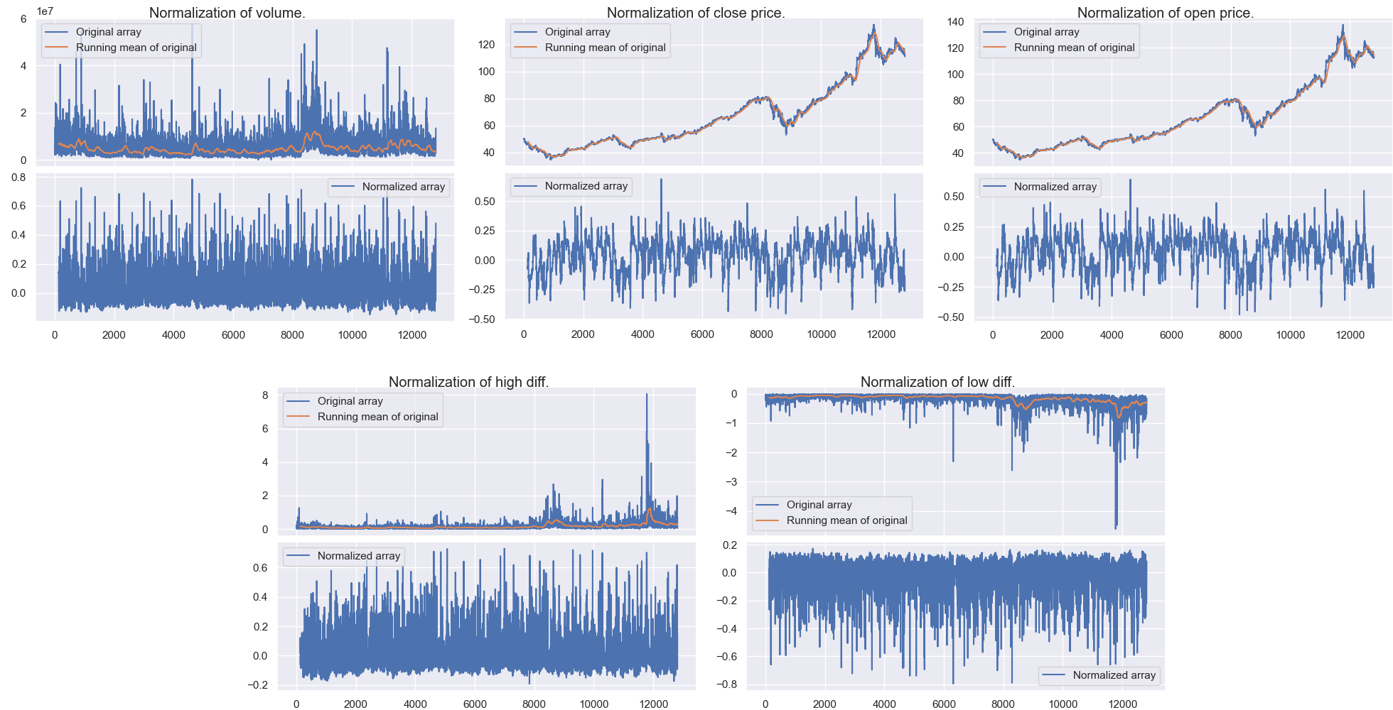
Normalization of the datapoint variables.
Table of contents:
Pipeline
The preprocessing pipeline consists of several stages. After the data has been sourced, it is processed through a series of stages. These are:
- Raw data gets loaded into memory.
- The data is trimmed down to normal working hours (09:30-16:00) since some of the equities list before/after-hour trading.
- The stocklabeler labels the data.
- RSI is calculated for the equity.
- The variables in each datapoint are normalized.
- Each end of the data is trimmed to remove edge-effects from running averages / convolutions.
- The data is saved as a csv file in data/training.
Window size:
The labeler uses “future” datapoints $P(t+ndt), n \in \mathbb{Z}^{+}$ to determine the label for a datapoint \(P(t)\). In practice, this is done using one or several convolutions depending on which labeling mode is used. Since the label is the only feature we wish to use future data to determine, the rest of the processing pipeline (normalization, RSI, …) must be restricted to previous datapoints \(P(t-n*dt)\). Because of the nature of discrete non-shifted convolutions, for any datapoint $P(t)$, values that are window_size/2 points away from the point in both directions are used. This means that for a window of 2 days, the labeler will look forward 1 day (and also 1 day backwards) when determining the label.
The choice of window size determines not only the investment period that we wish to train our network on, but also the results of technical indicators (such as RSI). If we set the window size to a 6 month period, we would target larger patterns than if we set it to 3 days since a bigger window would smooth out any small disturbances that are not relevant to this period.
Parameters
All the parameters used in the preprocessing stage can be found in the prep_config.py module in src/preprocessing/preprocessor. Below is a table of explanations and values used for the preprocessing stage using a window of 260 (one trading week look ahead):
| Parameter | Value | Description |
|---|---|---|
| $\texttt{DT}$ | 0.25 | Number of hours between each datapoint in the raw data. |
| $\texttt{LAB_CONV_FUNC}$ | ‘cubic’ | The convolution window to use for the labeler. |
| $\texttt{HOURS_AHEAD}$ | 32.5 | Hours ahead used to determine the label points. |
| $\texttt{HOURS_BEHIND}$ | 32.5 | Hours behind used in normalization. |
| $\texttt{THRESH_BUY}$ | 0.015 | Threshold for determining a buy point. |
| $\texttt{THRESH_SELL}$ | 0.015 | Threshold for determining a sell point. |
| $\texttt{MED_WIN}$ | 299 | Walking median window size for the custom labeler. |
| $\texttt{START_TRADE}$ | ‘09:30’ | Trading hours open time. |
| $\texttt{END_TRADE}$ | ‘16:00’ | Trading hours close time. |
| $\texttt{CLUSTER_SIZE}$ | 26 | Minimum size of the clusters to consider. The size n will result in images of size n x n. |
| $\texttt{REC_PERC}$ | 10 | nth percentile for which distances in the phase plot fall under are considered in the recurrence plot. |
| $\texttt{REC_DIST_MET}$ | ‘euclidean’ | Distance metric to use in the recurrence plots. |
| $\texttt{REC_ALPHA}$ | 15 | Factor used in the exponential grayscale mapping of the distances over the nth percentile in the recurrence plot. |
Note that since the networks where tested on two different sequence lengths, this table lists the parameters used for the sequence length of 260. For the data with sequence lengths of 52, $\texttt{HOURS_AHEAD}$ is set to 6.5 (one trading day) and $\texttt{THRESH_BUY}$ and $\texttt{THRESH_SELL}$ is set to 0.01. The reason for lowering the threshold values comes from the fact that a it is expected that a smaller window of investment means that each investment should yield a smaller absolute profit. Therefore, the threshold values should reflect this.
Normalization
Normalizing the data before feeding it into the neural network can increase the performance of the network. Financial data can be hard to normalize, and there are many approaches to take when doing so. First comes the determination of what to normalize, then comes the determination of how to normalize it. We could for example choose to normalize the closing price of a stock C(t) for some time t, but we would then need to determine how this is to be normalized. Extra care must also be taken so that no future information is incorporated into the normalizattion process.
Why normalize in the first place?
From a technical perspective, normalizing the data before training can have drastic effects on training times. Multiple algorithms have shown to converge faster for data that in a small range. While training using gradient decent, one might encounter exploding gradients if the features of the instance are grossly disproportionate.
Normalization can also have severe effects on the performance of neural networks. In Efficient approach to Normalization of Multimodal Biometric Scores, the authors present multiple methods and the effects on them in neural networks. A popular normalization method is the modified tanh estimator. This has the advantage of using the standard deviation and mean of the dataset instead of using the Hampel estimators. It is thus faster and simpler than the normal tanh estimator, but has the same qualities such as robustness. The modified tanh estimator is given by
How was the data normalized?
The modified tanh normalizer was again modified to yield an output range of [-1, 1] and a mean of 0. The expression for this version is
This new modified version also ensures that values within one standard deviation at maps to around [0.1, 0.1]. For the lack of a better name, lets call this the modified modified tanh normalizer. This was applied on all the data except for the RSI value which was divided by 100 (theoretical maximum value of the RSI). For the high and low price, these where first calculated to their differences from the average price within the 15 minute period. That is
and